Finding the Shortest Path from Source to other Nodes

Breadth-first-search (BFS) is an algorithm for traversing or searching tree or graph data structures. It starts at the tree root (or some arbitrary node of a graph, sometimes referred to as a ‘search key’) and explores the neighbor nodes first, before moving to the next level neighbors. BFS was invented in the late 1950s by Edward Forrest Moore, who used it to find the shortest path out of a maze and discovered independently by C. Y. Lee as a wire routing algorithm in 1961.

The processes of BFS algorithm works under these assumptions:

1. We won’t traverse any node more than once.
2. Source node or the node that we’re starting from is situated in level 0.
3. The nodes we can directly reach from source node are level 1 nodes, the nodes we can directly reach from level 1 nodes are level 2 nodes and so on.
4. The level denotes the distance of the shortest path from the source.

Let’s see an example:

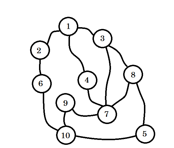
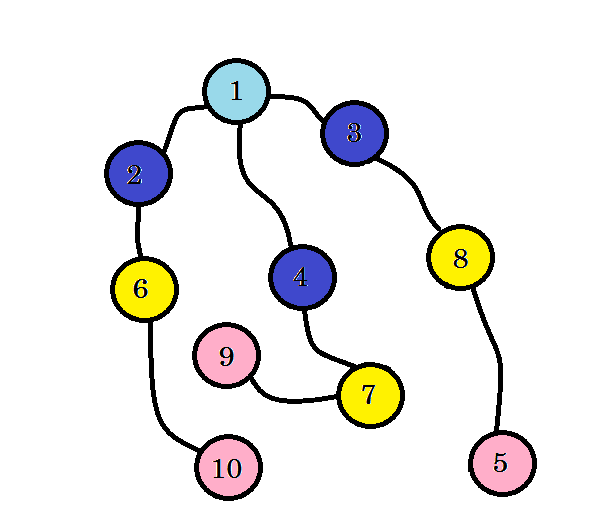
Let’s assume this graph represents connection between multiple cities, where each node denotes a city and an edge between two nodes denote there is a road linking them. We want to go from node 1 to node 10. So node 1 is our source, which is level 0. We mark node 1 as visited. We can go to node 2, node 3 and node 4 from here. So they’ll be level (0+1) = level 1 nodes. Now we’ll mark them as visited and work with them.

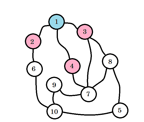
The colored nodes are visited. The nodes that we’re currently working with will be marked with pink. We won’t visit the same node twice. From node 2, node 3 and node 4, we can go to node 6, node 7 and node 8. Let’s mark them as visited. The level of these nodes will be level (1+1) = level 2.

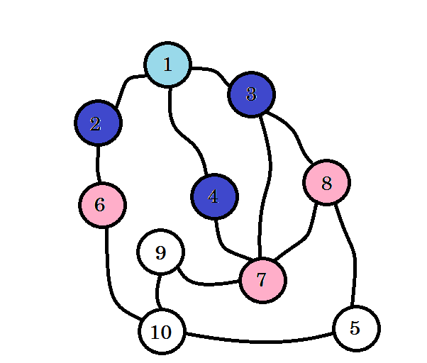
If you haven’t noticed, the level of nodes simply denote the shortest path distance from the source. For example: we’ve found node 8 on level 2. So the distance from source to node 8 is 2.

We didn’t yet reach our target node, that is node 10. So let’s visit the next nodes. we can directly go to from node 6, node 7 and node 8.

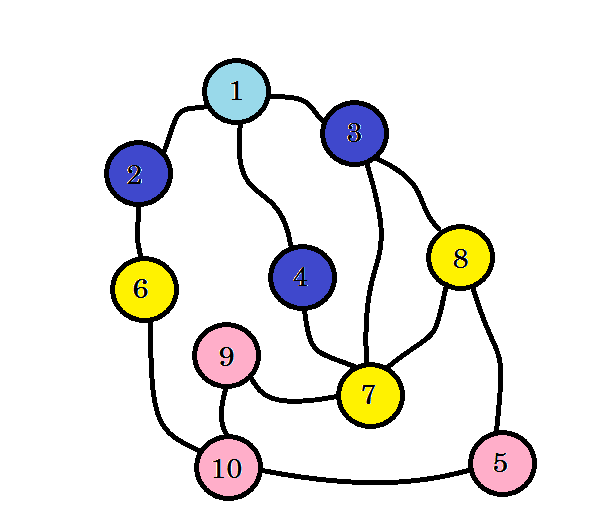
We can see that, we found node 10 at level 3. So the shortest path from source to node 10 is 3. We searched the graph level by level and found the shortest path. Now let’s erase the edges that we didn’t use:

After removing the edges that we didn’t use, we get a tree called BFS tree. This tree shows the shortest path from source to all other nodes.

So our task will be, to go from source to level 1 nodes. Then from level 1 to level 2 nodes and so on until we reach our destination. We can use queue to store the nodes that we are going to process. That is, for each node we’re going to work with, we’ll push all other nodes that can be directly traversed and not yet traversed in the queue.

The simulation of our example:

First we push the source in the queue. Our queue will look like:

front
+-----+
|  1  |
+-----+

The level of node 1 will be 0. level[1] = 0. Now we start our BFS. At first, we pop a node from our queue. We get node 1. We can go to node 4, node 3 and node 2 from this one. We’ve reached these nodes from node 1. So level[4] = level[3] = level[2] = level[1] + 1 = 1. Now we mark them as visited and push them in the queue.

front
+-----+  +-----+  +-----+
|  2  |  |  3  |  |  4  |
+-----+  +-----+  +-----+

Now we pop node 4 and work with it. We can go to node 7 from node 4. level[7] = level[4] + 1 = 2. We mark node 7 as visited and push it in the queue.

front
+-----+  +-----+  +-----+
|  7  |  |  2  |  |  3  |
+-----+  +-----+  +-----+

From node 3, we can go to node 7 and node 8. Since we’ve already marked node 7 as visited, we mark node 8 as visited, we change level[8] = level[3] + 1 = 2. We push node 8 in the queue.

front
+-----+  +-----+  +-----+
|  6  |  |  7  |  |  2  |
+-----+  +-----+  +-----+

This process will continue till we reach our destination or the queue becomes empty. The level array will provide us with the distance of the shortest path from source. We can initialize level array with infinity value, which will mark that the nodes are not yet visited. Our pseudo-code will be:

Procedure BFS(Graph, source):
Q = queue();
level[] = infinity
level[source] := 0
Q.push(source)
while Q is not empty
    u -> Q.pop()
    for all edges from u to v in Adjacency list
        if level[v] == infinity
            level[v] := level[u] + 1
            Q.push(v)
        end if
    end for
end while
Return level

By iterating through the level array, we can find out the distance of each node from source. For example: the distance of node 10 from source will be stored in level[10].

Sometimes we might need to print not only the shortest distance, but also the path via which we can go to our destined node from the source. For this we need to keep a parent array. parent[source] will be NULL. For each update in level array, we’ll simply add parent[v] := u in our pseudo code inside the for loop. After finishing BFS, to find the path, we’ll traverse back the parent array until we reach source which will be denoted by NULL value. The pseudo-code will be:

Procedure PrintPath(u):  //recursive    |   Procedure PrintPath(u):   //iterative
if parent[u] is not equal to null       |   S =  Stack()
    PrintPath(parent[u])                |   while parent[u] is not equal to null    
end if                                  |       S.push(u)
print -> u                              |       u := parent[u]
                                        |   end while
                                        |   while S is not empty
                                        |       print -> S.pop
                                        |   end while

Complexity:

We’ve visited every node once and every edges once. So the complexity will be O(V + E) where V is the number of nodes and E is the number of edges.